After completing this lesson, learners should be able to:
Understand that a pixel index is related to a physical coordinate.
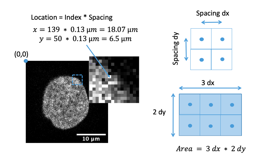
Understand that a spatial calibration allows for physical size measurements.
Motivation
We would like to relate the image dimensions to a physical size. The relation between pixels and physical size is referred to as spatial calibration. Image calibration is dictated by acquisition and detection parameters of a microscope, such as magnification, camera detector size, sampling, etc, and is usually stored within the so-called image metadata. Before performing quantitative measurements, e.g. volume, area, …, you should make sure that the spatial calibration has been set appropriately.
Concept map
graph TD
Im("Image") --> P("Pixels")
Im --> C("Calibration")
P --> Va("Value")
P --> I("Indices")
I --> CC("Calibrated coordinate")
C --> CC
Figure
Spatial calibration and size measurements
Isotropy
One speaks of isotropic sampling if the pixels have the same extent in all dimensions (2D or 3D).
While microscopy images typically are isotropic in 2D they are typically anisotropic in 3D with coarser sampling in the z-direction.
It is very convenient for image analysis if pixels are isotropic, thus one sometimes resamples the image during image analysis such that they become isotropic.
Open one of the above images using Plugins › Bio-Formats › Bio-Formats Importer
[X] Display OME-XML metadata
Find the pixel calibration in the metadata text
Also inspect the pixel size in Image > Properties
Check that those information are consistent
Add a scale bar to the image using Analyze › Tools › Scale Bar...
Explore the various options for where and how to place the scale bar
Export the image using Plugins › BioVoxxel Figure Tools › Export SVG (requires BioVoxxel update site)
SVG preserves the rendering of the scale bar at different zoom levels.
Open the raw data image again using File > Open... instead of Bio-Formats
Are you getting the same pixel calibration?
ImageJ Macro
// Open image using Bio-Formats//// Unfortunately, Bio-Formats cannot read commercial file formats from an URL: https://forum.image.sc/t/open-url-with-bio-formats/85074// Thus, please download any image specified in the activity and replace "Path_to_your_image" in the below coderun("Bio-Formats Importer","open=[Path_to_your_image] display_metadata display_ome-xml");// As macros cannot directly read the text from the metadata window, // We skip the part about reading from the metadata text window,// which has to be done manually.// Get pixel width and height from propertiesgetPixelSize(unit,pixelWidth,pixelHeight);print("Unit =",unit);print("pixelHeight= ",pixelHeight);print("pixelWidth",pixelWidth);// Add scale bar to the image//// Please experiment with the parameters to change the scale bar overlayrun("Scale Bar...","width=100 height=5 font=12 color=White background=None location=[Lower Right] overlay");
Appreciate that image calibration might be necessary, e.g.
2D distance measurement between two pixels
One can use the Line tool
3D distance measurement between two voxels
One cannot use the Line tool but needs to measure manually: sqrt( (x0-x1)^2 + (y0-y1)^2 + (z0-z1)^2 )
Note: It is critical to use the calibrated voxel positions and not the voxel indices in above formula!
Appreciate that image calibration can be confusing, e.g.
It is not consistently used in image filter parameter specification
skimage napari
# %%
# Spatial image calibration
# %%
# Import python packages
fromOpenIJTIFFimportopen_ij_tiffimportnumpyasnpfromnapari.viewerimportViewer# %%
# Open a 3-D image of metaphase chromosomes and inspect the metadata
image,axes,voxel_size,units=open_ij_tiff("https://github.com/NEUBIAS/training-resources/raw/master/image_data/xyz_8bit__mitotic_plate_calibrated.tif")print("Shape:",image.shape)print("Axes:",axes)print("Scale:",voxel_size)# anisotropy!
print("Units:",units)# %%
# View the image in napari
viewer=Viewer()viewer.add_image(image)# Napari:
# - Change the axes order to look at the image "from the side" using the corresponding button
# - Look at the image in 3-D using the corresponding button
# - Conclude that the physical shape does not look correct
# - Important: close this viewer before proceeding, not to confuse yourself
viewer.close()# %%
# Open napari and add the image with its voxel size.
viewer=Viewer()viewer.add_image(image,scale=voxel_size)# %%
# Napari GUI: Change the viewer dimension order using the corresponding button.
# Napari GUI: Use the 3D viewer button to render the image in 3D.
# %%
# Compute distances between points
#
# Napari GUI: use the `New points layer button` to create a new points layer.
# Napari GUI: use `Add points` to add two points somewhere on the meta-phase plate.
# %%
# Napari:
# - Again look at the image from the side and in 3-D
# - Observe that, thanks to the "scale", the 3-D physical shape looks correct now
# - Observe that napari added interpolated data to make the image appear scaled
# %%
# In the following, we will compute distances between 3-D points
# This is interesting, as you will learn:
# - How to use drawing layers in napari
# - How to use image scaling (voxel_size) information for physical measurements
# %%
# Extract the point coordinates
points=viewer.layers['Points'].dataprint(points)# unscaled => not very useful for physical measurements
# %%
# Scale the points
scale=viewer.layers['Points'].scale# same as voxel_size
print("Points scale: ",scale)print("Voxel size: ",voxel_size)points_cal=points*scaleprint("Points:\n",points)print("Calibrated points:\n",points_cal)# %%
# Compute the distance between the first and second point
print("First point:",points_cal[0])print("Second point:",points_cal[1])fromscipy.spatialimportdistancedistance.euclidean(points_cal[0],points_cal[1])# %%
# Close the viewer (CI test requires this)
viewer.close()
Open xyz_8bit__nucleus.tif and add the spatial calibration in x & y of the previous image; add a voxel-depth of 0.52 um.
Measure the length of the longest axis of the nucleus.
Show activity for:
ImageJ GUI
[File > Open ] the image and then [Image > Properties …] or [Ctrl-Shift-P]. Pixel-height = pixel-width = 0.13 um.
Open the 3D image and change the properties from the [Image > Properties …] gui and the unit.
Maximal extension is ~ 19.2 um. Move to the middle of the nucleus (~ z-slice 3) and draw a line using the line-tool.
skimage napari
# %%
# ## Spatial image calibration
# %%
# Import python packages.
importosfromOpenIJTIFFimportopen_ij_tiff,save_ij_tifffromnapari.viewerimportViewerimportnumpyasnp# %%
# Open a 2D image and its axes metadata
image_2D,axes_image_2D,voxel_size_image_2D,units_image_2D=open_ij_tiff("https://github.com/NEUBIAS/training-resources/raw/master/image_data/xy_8bit__nucleus_calibrated.tif")# %%
# Inspect the image metadata
print("Shape: ",image_2D.shape)print("Axes: ",axes_image_2D)print("Scale: ",voxel_size_image_2D)print("Units: ",units_image_2D)# %%
# Open a 3D image and its axes metadata
image_3D,axes_image_3D,voxel_size_image_3D,units_image_3D=open_ij_tiff("https://github.com/NEUBIAS/training-resources/raw/master/image_data/xyz_8bit__nucleus.tif")# %%
# Inspect the image axes metadata.
print("Shape: ",image_3D.shape)print("Axes: ",axes_image_3D)print("Scale: ",voxel_size_image_3D)print("Units: ",units_image_3D)# %%
# Note that the 3D image does not have calibrated metadata.
# Let's add spatial calibration using the x&y voxel_size from the 2D image
# and also add a z scaling
voxel_size_image_3D=[0.52,voxel_size_image_2D[1],voxel_size_image_2D[0]]units_image_3D=["um","um","um"]# %%
# Inspect the metadata for the 3D image
print("Shape: ",image_3D.shape)print("Axes: ",axes_image_3D)print("Scale: ",voxel_size_image_3D)print("Units: ",units_image_3D)# %%
# Open napari and add the 3D image with voxel_size
viewer=Viewer()viewer.add_image(image_3D,scale=voxel_size_image_3D,name='image_3D')# %%
# Napari GUI: Use the 3D viewer button to render the image in 3D.
# %%
# Save the 3D image with the calibration metadata
save_ij_tiff(# during trainings this Path should be replaced by the user's desktop, e.g. C:/Users/dominik/Desktop
os.path.join(os.path.expanduser("~"),"image_3D_calibrated.tif"),image_3D,axes_image_3D,voxel_size_image_3D,units_image_3D)# %%
# Open the above file in FIJI and verify image scales were properly saved.
# %%
# Measure the length of the nucleus (as exercise)
# Napari GUI: use the `New points layer button` to create a new points layer.
# Napari GUI: use `Add points` to add two points along the longest axis
# %%
# points = napari_viewer.layers['Points'].data
# scale = napari_viewer.layers['Points'].scale
# points_cal = points * scale
# print("Points :\n", points)
# print("Calibrated points :\n", points_cal)
# %%
# from scipy.spatial import distance
# distance.euclidean(points_cal[0], points_cal[1])
# %%
# Close the viewer (CI test requires this)
viewer.close()
Assessment
Answer these questions
Given a 2D image with pixel height = pixel width = dxy = 0.13 micrometer, what distance do the pixels at the (x,y) indices (10,10) and (9,21) have in micrometer units?
Given a 3D image with dx = dy = 0.13 micrometer and dz = 1 micrometer, what is the calibrated (micrometer units) distance of two pixels at the indices (10,10,0) and (9,21,3)?
What is the calibrated (micrometer units) area covered by 10 pixels, given a spatial calibration of dx = dy = 0.13 micrometer?
What is the calibrated (micrometer units) volume covered by 10 voxels, given a spatial calibration of dx = dy = 0.13 micrometer and dz = 1 micrometer?
Solution
sqrt( (x0*dxy-x1*dxy)^2 + (y0*dxy-y1*dxy)^2 ) = sqrt( (x0-x1)^2 + (y0-y1)^2 ) * dxy = sqrt( (10-9)^2 + (10-21)^2 ) * 0.13 = 11.04536 * 0.13 micrometer = 1.435897 micrometer. The fact that one can separate out the isotropic calibration dxy in the formula allows one to perform measurements in pixel units and convert the results to calibrated units later, by means of multiplication with dxy.
sqrt( (x0*dx-x1*dx)^2 + (y0*dy-y1*dy)^2 + (z0*dz-z1*dz)^2 ) = sqrt( (10*0.13-9*0.13)^2 + (10*0.13-21*0.13)^2 + (0*1.0-3*1.0)^2 ) micrometer = 3.325928 micrometer. Unfortunately, in an anisotropic 3D image one cannot separate out a calibration factor from the formula, making life more difficult.
10 * 0.13 micrometer * 0.13 micrometer * 1.0 micrometer = 10 * 0.0169 micrometer cube = 0.169 micrometer cube. This shows that measuring volumes in 3D can be done first in voxel units, as the calibration factor can easily taken into account later (in contrast to the distance measurements). Thus, somewhat surprisingly, is in practice easier to measure volumes than distances in 3D.